Updated April 11, 2022. This article is being continuously expanded, amended and improved. For the log of major changes, see the changelog.txt.
The subject of sound in home computers is fascinating, and the decade between mid 1980s and mid 90s saw a fierce competition of digital sound representation methods, sound processing chips, and manufacturers. This article is the result of my attempt to re-discover and understand the technologies behind sound reproduction in computers. Where available, I will be using actual products from that era. The article was greatly inspired by previous works by Piotr Gontarczyk (here), Stefan Goehler (here) and countless other printed and online resources. For details see the Reference section.
There is a series of videos accompanying this article. If you prefer watching to reading, here is the intro episode:
Sound is a mechanical agitation of air which takes the form of waves. It is produced by living organisms and things, transported through the air for a limited distance, and potentially received by other organisms or things. To increase sound transport distance, to store it for reproduction at a later time, or to create new artificial sounds, methods have been devised to transform acoustic waves into electric impulses. The transportation and storage can be analog (acoustic waves are represented as electric waves), or digital (acoustic waves are represented as series of bits). Analog representation is continuous (sound does not need to be broken up into pieces) while digital representation is discreet (waves are "probed" — sampled — at certain points and these snapshots are stored or transported). The advantage of the former is (theoretically) higher fidelity to the original sound while the advantage of the latter is higher reliability and easier storage and transformation of sound. In practice, with today's technology advancements digital representation also meets high fidelity requirements.
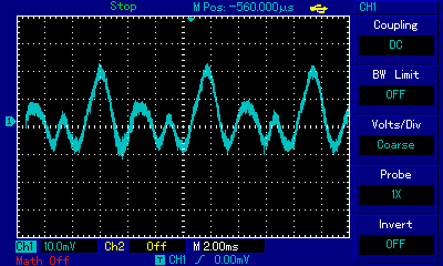
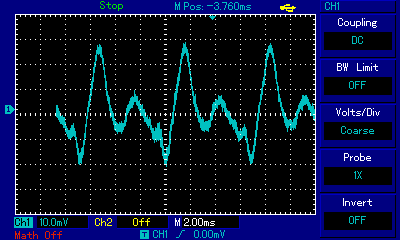
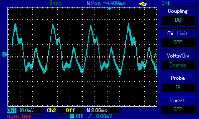
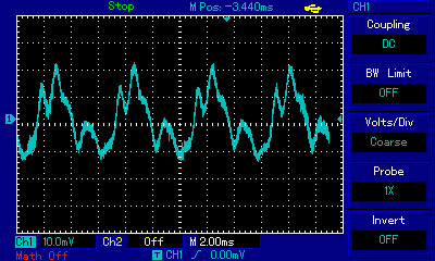
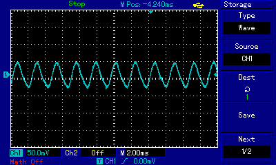
Now, let's try and experiment before we move on. Oscilloscope helps us observe the sound waves in their raw form. The oscilloscope I'm using is digital, so there is a digital transformation before the wave is displayed, but we can ignore that — we could just as well be using an old analog oscilloscope. What I'm saying is that we can "see" the sound wave before it is digitized in any way. Like below, when we play the C major scale on the acoustic guitar. Let's listen first:
And then look at the waves:
Electric guitar is just that: electric. It sounds different, and waves are transmitted over a cable instead of air, but it is still analog, not digital.
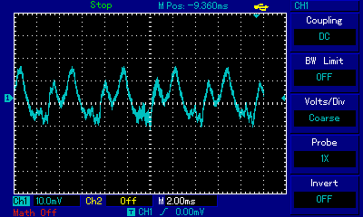
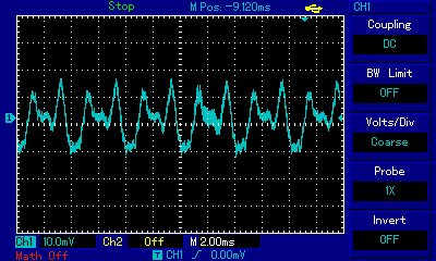
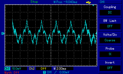
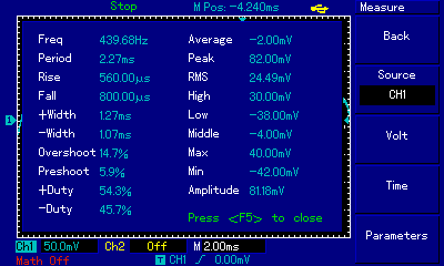
Look at the periods of the waves above. One square on the horizontal scale corresponds to 2 milliseconds, i.e. 2 thousands of a second. So the period (horizontal span at which the wave's shape starts to repeat) for the note C above seems close to 0.008s or 0.009s. Then the period decreases with every note of the scale played, and for A above it is down to somewhere between 0.004s and 0.005s. We know that frequency of a wave is the inverse of its period, so we calculate the frequency of A at somewhere between ≈1/0.004 = 250Hz and ≈1/0.005 = 200Hz (hertz means "agitations per second"). In fact, the note A4 is officially defined as 440Hz which is twice the frequency of what we measured. Twice, because our sound was A3, i.e. an octave lower.
Waves illustrated above are not too similar to the well-known sine wave ∿ we all know from school. The reason is that traditional instruments produce much more sound than just the base note. There are additional harmonic components in the waves produced, resonance from other parts of the instrument (e.g. other strings), as well as noise components (e.g. caused by imprecise string plucking, scratching the string with fingernail, etc.). Also, the intensity (amplitude) of sound, and the presence of these additional components, is not the same throughout the lifetime of the sound.
By the way, you don't need to buy a real oscilloscope if you don't have one. If you don't mind some digital processing, delay and inaccuracies, you can make similar experiments using the online Virtual Oscilloscope.
Click below for the video record of my exercises with sound waves...
At a low level, computers process data in binary form: either true, or false; either 1 or 0. Only two extreme values. This is the exact opposite of any analog signal where in addition to the two extremes there can also be an infinite number of intermediate values. And that is why the whole subject of converting between these two representations is so interesting, and why we have this article in the first place.
By early 70s it had become obvious that home computers had to have some means of communicating messages — for example errors or acknowledgements – in audio as well as visual form. But they were not equipped with digital-to-audio (DAC) converters, so methods were devised to simulate the analog signal with digital ("1" or "0") impulses. Let's try and understand these techniques by re-creating them using Arduino. To run the following experiments on your own, all you need is any Arduino board, a couple of resistors, any small speaker (e.g. 0.25W which was typical in the PCs of the 80s and 90s), and optionally a LED (to understand when the speaker is on, and when off) and potentiometer. You also need Arduino software for your computer in order to upload the sketches we discuss below to your Arduino.
The Arduino examples described below are also covered in the following video:
Let's connect the speaker to Arduino in the following way:
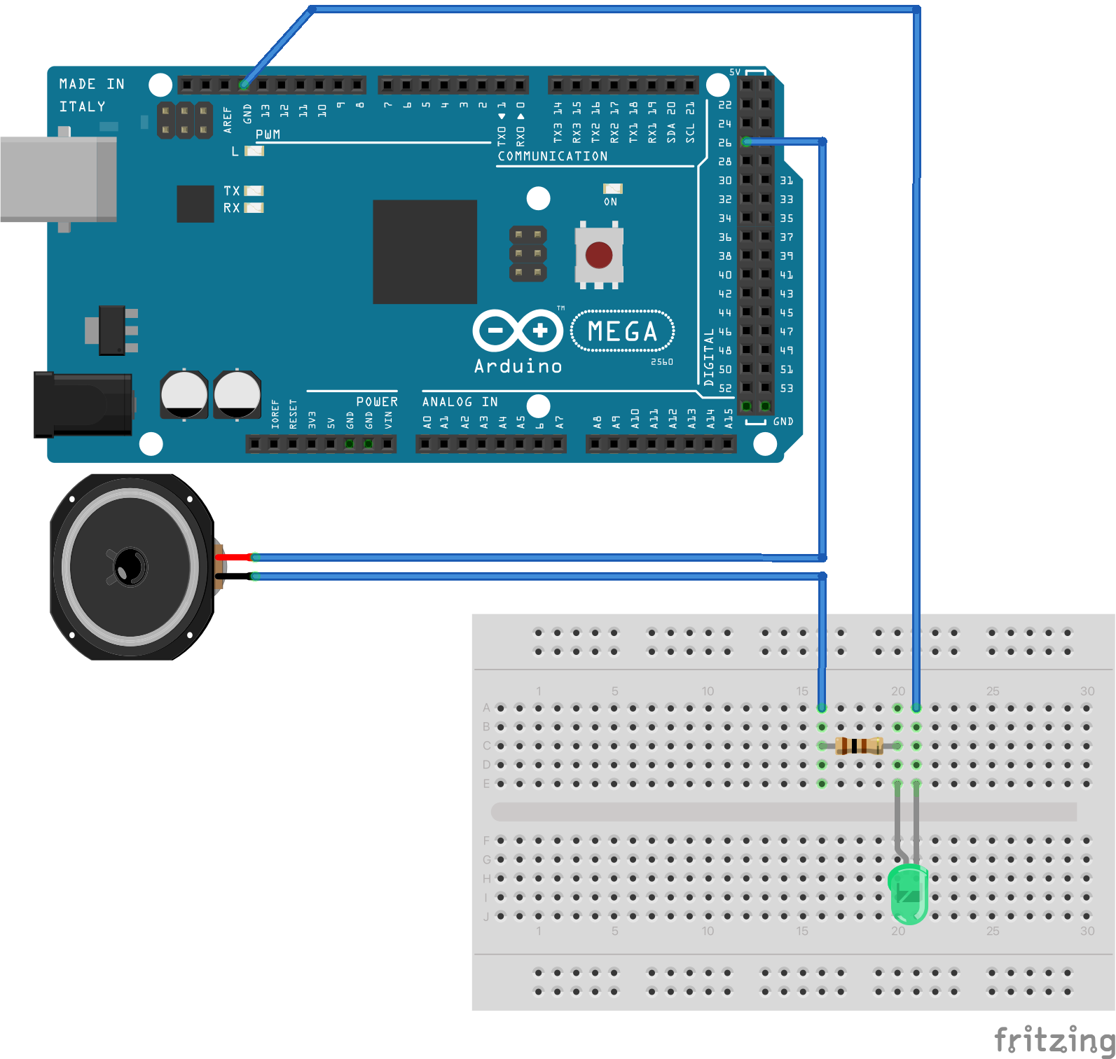
Now if we upload and run the following code, the speaker will star ticking twice a second. How is that happening? We're applying voltage to the speaker which energises the speaker's driver and pushes the membrane out, making a ticking sound. After waiting 500 milliseconds we're we're disconnecting the voltage; the driver's electromagnet is not energized anymore and the membrane gets pulled back in, making another ticking sound. The "out" and "in" sounds are almost indistinguishable, and both of them together constitute one "on"/"off" cycle. Here is what it sounds like:
And below is the code responsible for that effect:
Continuous sound can be generated by increasing the frequency of the ticks, i.e. decreasing the delays between them. Here is what A4 note sounds like if generated that way.
And here is the Arduino code which generated it. Check out the interdependencies between period (the two delays in one cycle combined) and frequency.
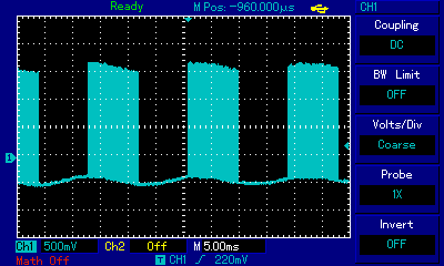
That said, the generated wave is not at all like the one coming from a real instrument. Compare the close-to-sine sound wave (blue) generated by a guitar and and the on/off square wave generated by the piece of code above.
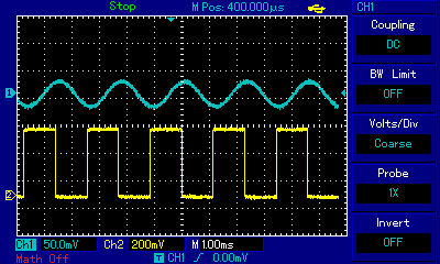
The frequency is the same, but the shape is different, and the difference is clearly distinguishable by the human ear. The shape of a sound wave dictates its timbre which is a quality distinct from pitch and intensity. Later we will see how other sound synthesis methods tried to overcome the limitation of the binary, or "on/off only", quality of 1-bit speaker.
Square wave produces a characteristic "beep" sound which has been used in many devices to communicate alerts, acknowledgements, and errors to users. In computers, the beep sound history reaches back all the way to mainframe terminals where a special character, bell, was used to denote alert condition (which, in turn, had its origins in the ring sound of a typewriter denoting the end of line). The bell code, even though it represents a sound, remains a part of ASCII character set, and one can actually embed it in a file, or even type it in by pressing Ctrl+G in any modern terminal emulator, e.g. in Linux or macOS. In the 80s the square-wave beep — by far the cheapest method to produce sound in electronic devices — became so ubiquitous that some programming languages made the BEEP command a part of their standard libraries. Examples are ZX Spectrum 48K built-in BASIC interpreter and even some programmable calculators! Here are sound samples generated on a HP 28S Advanced Scientific Calculator. Since the calculator uses Reverse Polish Notation (RPN), instead of typing in BEEP 3, 9 (3-second A note) as we would in ZX Spectrum, we need to type in 220 3 BEEP. Here is the A note played on an HP 28S across 4 octaves: 220Hz, 440Hz, 880Hz, 1760Hz (each subsequent octave doubles the frequency of a note):
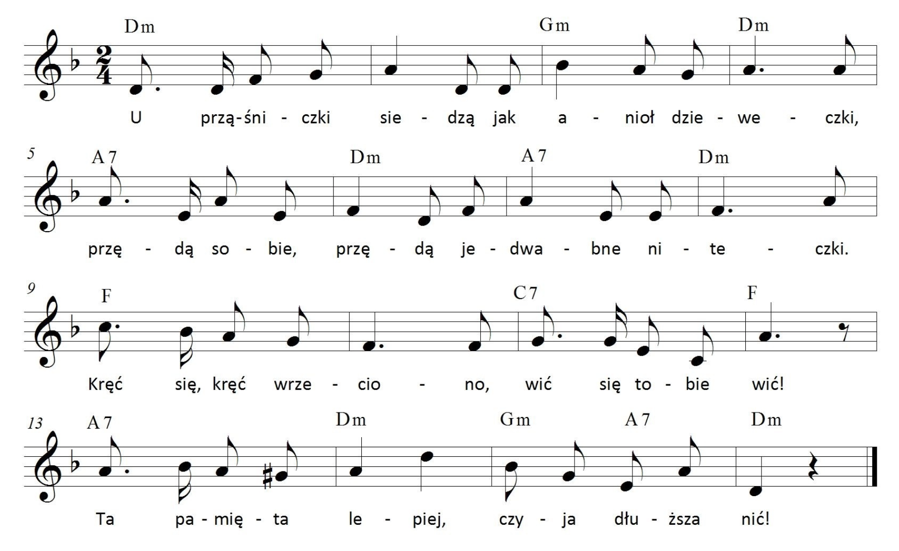
So at this point nothing stops us from playing a tune, i.e. sequence of sounds of specific length and pitch. In the code below we took a Polish tune from 19th century titled Prząśniczka and transcribed it as a series of frequencies and lengths. 0.2 corresponds to an eigth note, 0.4 to a quarter note, 0.3 to a dotted eight, and so on. Frequencies corresponding to note pitches can be found here.
Here is what it sounds like. Note that some of the pitches are difficult to get right because of other factors to Arduino processing, in particular the calculations it has to do with every loop iteration. If you want pitches closer to perfect, use Arduino's built-in tone() function. It uses the actual Arduino's timers to get the right frequencies, and hides many complexities, but for the sake of our discourse I deliberately refrained from using it.
Since a PC speaker provides just one sound channel, there is no way to play chords (multiple notes played at the same time). But there are ways to simulate chords by cheating the human ear. Arpeggio is one of them; in music world it just means playing several notes in quick succession as a form of artistic expression; but in early computer music arpeggios were played fast to create the impression of chords. Listen to chords C major, A minor, D minor, G major simulated by playing arpeggios of respectively (C, E, G); (A, C, E); (D, F, A); (G, H, D) notes, with each note played for 6 hundredths of a second.
See the code responsible for this pleasant noise:
In all the examples above the ratio between the "on" and "off" states of the speaker was 1:1, i.e. 50% of the time the speaker was "on" and 50% of time the speaker was "off". This is called 50% duty cycle of a square wave. It turns out that certain properties of sound generated by square wave will change — even if we don't change the frequency itself — when duty cycle is modified. So if we apply voltage to the speaker for 20% of the time, and leave it off for 80% of the time, the sound will retain the same frequency as in 50/50 duty cycle, but the timbre will change. In this sample, we first increase the sound frequency, and then (around 0:22s) modulate the duty cycle. We then change frequency again, and modulate duty cycle again, repetitively. Hear how the perception of sound changes from more "ripe" or "full" to "shallow" or tinny" and vice versa when modulating the duty cycle.
Below are the Arduino setup and sketch I used to simulate the above frequency and duty cycle modulations with 3 potentiometers (one for coarse frequency tuning, another one for fine frequency tuning, and a third one for duty cycle modulation).
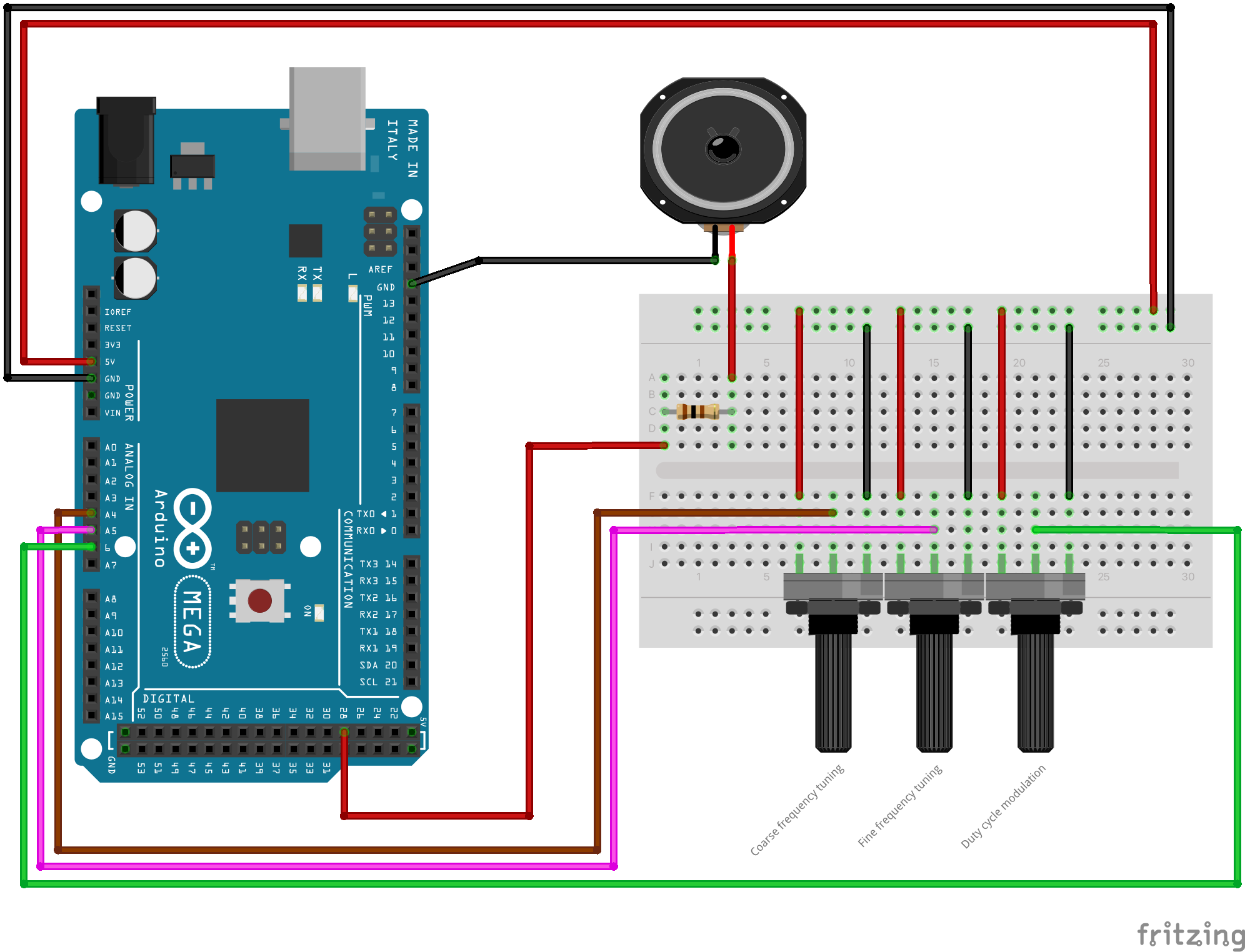
The techniques of controlling the frequency and duty cycle of a square wave are called Pulse Width Modulation (PWM), and are applied to many fields of computing and communications as well as computer sound. For the use in sound, 1-bit speaker and PWM techniques were — and still are — used extensively in many early home computers, including PCs, Apple II, ZX Spectrum, and other computing and non-computing devices like calculators, dumb terminals, and household appliances. Let's look at how the idea was implemented in ZX Spectrum, Apple II, and PCs.
Even though we just put ZX Spectrum, Apple II and the early PCs in one bucket — let's call it 1-bit music generators — in fact there are differences between these platforms in how they drive that 1-channel speaker. In particular, while in the PCs the speaker is connected to a PIT (programmable interval timer) which only then is driven by the CPU, in both ZX Spectrum and Apple II the speaker is driven directly by the CPU. As a consequence, the CPUs of the two latter machines are much busier when generating sound than the PC CPU is. This has severe implications on how software was written for these platforms: code which did something else had to be executed in a disciplined manner to fit the precisely timed speaker clicks. This required a lot of ingenuity. If you prefer watching, click below to see the video which covers some of the subjects covered in this Apple II section:
Let's listen to a few examples of Apple II software using sound routines. The first one, Family Feud game published by Sharedata in 1984, simply stops all processing to play the initial tune:
With the exception of evenly spaced noise outbursts which outline the rhythm, there is nothing unusual here: a pulse train of various frequencies, all employing 50-percent duty cycle. Similarly in the next track from the game Frogger by Konami/SEGA, whose Apple II port was released in 1982, only 50-percent duty cycle square wave was used, but with a very well composed alternation between two melodies, one in the lower register and one in the higher one, which creates a pleasing counterpoint effect.
Interestingly enough, the Frogger game is about a frog, but intro tune is based on an old Japanese nursery rhyme which tells a story of a cat and dog...
As mentioned, in non-expanded Apple II there was no way to leave sound playing while engaging the CPU with other tasks. Each single speaker click required a CPU cycle, and to play the simplest A3 sound using square waves for only 1/5th of a second, 880/5 = 176 such CPU cycles are needed! (And that's just CPU work on clicking the speaker, not to count looping, decrementing counters, etc.) It should not be surprising that many devs settled on the simplest solution like the one used in Family Feud above: don't do anything else while sound is playing. Yet there were notable exceptions, one of them being Ms. Pac-Man, a 1982 game by General Computer Corporation and relased for Apple II by Atarisoft, where well-designed character sounds and tune snippets were incorporated into the game without stopping the gameplay at all (e.g. when Ms Pac-Man is eating the dots) or with minimal slowdown (e.g. when Ms Pac-Man devours a ghost). The game's soundtrack was well thought-through in all aspects; even the short initial tune is not just a square pulse train but a very clean two-sound harmony.
Namco's 1981 game Dig Dug, ported to Apple II in 1983, is amazing in even playing a melody in game, while the character was moving on the screen and doing things! Here is what it sounds like:
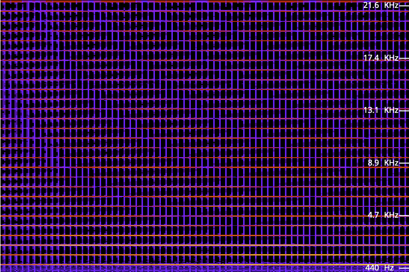
[... Dig Dug sound...]As we move away from the 50-percent duty cycle, a good idea is to explore the auditory implications of using very narrow rectangular waves, i.e. ones of very low or very high duty cycle. In short, as the duty cycle approaches 0% (or 100%), the harmonic components are more evenly distributed, without the fundamental one strongly dominating which, in turn, means that a long tail of harmonic components are lost beyond human hearing ability, and beyond hardware frequency response, so relatively less of the specific sound can be heard. To explore the behavior of very low-duty cycle rectangular waves at different frequencies, I wrote a simple assembly program for the Apple II where the user is able to modulate frequency of the continuous sound with a pair of keys (arrows left and right), and modulate the duty cycle with another pair of keys (A and Z). Here is what modulating the duty cycle sounds like, and how frequency distrubution changes. Pay attention to the tall red line to the very left of the image. It represents the fundamental harmonic, and it is less and less dominating as the pulse width gets thinner:
Here is the assembly code of my program:
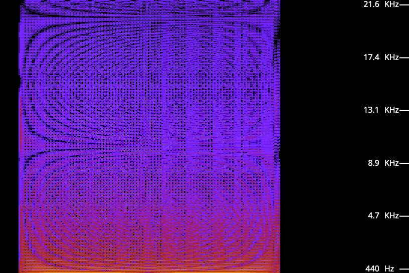
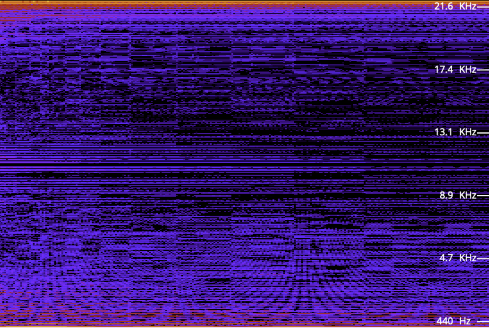
Another way of looking at the effect of thin pulses is to examine the spectrogram of the progression from very low to 50-percent duty cycle. Again using my simple program I was able to generate approx. 780Hz frequency and gradually modulated the duty cycle from a very thin pulse to 50%. Listen to, and look at, the effect of this:
The 1981 game Defender uses that gradual modulation of duty cycle a lot, and the resulting spectrogram looks like a work of abstract art:
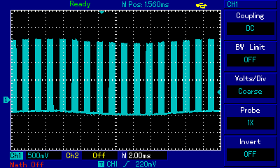
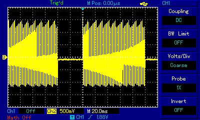
The volume modulating effect of harmonic composition of low-duty cycle square waves on sound power was applied for example in Oscillation Overthruster, an interesting Apple II program published by David Schmenk in 2017. In Oscillation Overthruster, the sound power modulation effect was used to shape (albeit in a crude way) the ADSR (attack, delay, sustain, release) envelope of sound which is really crossing the boundaries of the platform as being able to control such envelopes pertain to much more advanced chips which we will discuss later. To achieve this control, Oscillation Overthruster starts with a very thin rectangular pulse; here is what C Major scale sounds like, and looks like, when played in this program:
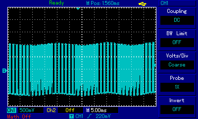
The sound sample and the animated gif show us walking over the C Major scale from C3 (approx. 7.6ms ≈ 131Hz) to C4 (3.8ms ≈ 263Hz). One can immediately notice that the rectangular pulses generating these frequencies are extremely thin; on this 2ms scale looking very much like lines. And yet as the sound fades, the pulse gets even thinner. Let's zoom in on a single pulse in the pulse train for the note A3:
We can observe that the pulse width starts at around 70µs (that's microseconds) which for the note A3 (220Hz ≈ 4.54 miliseconds) is barely 1.5% of the wavelength! And then it only gets thinner as the sound fades, all the way to less than 20µs (0.4%), before desappearing altogether. In reality the pulses (signal high) are actually very wide and the spacing between them very thin (signal low), but for the aural expression using rectangular waves the spacing can be treated as pulses and vice versa. It is of little meaning whether we are dealing with a 1.5%-wide crest and 98.5%-wide trough or the other way round. A different thing should immediately shout at us from the above gif: it is the shape of the pulse. While initially it still bears some resemblance to rectangle (even though already rounded), as it gets thinner it completely loses its rectangular features and starts resembling a triangle. To understand this, we first need to look at the scale of the oscilloscope view. One square is 50µs wide, so the leaning slope of the wave is somewhere around 10µs wide. That's 1/100,000 of a second. If we zoom out to a scale more appropriate for representing sonic frequencies (e.g. 2ms per square), that leaning line will look perfectly straight, and for all purposes it will behave as if the time to switch between high and low state was infinitesimal. Limitations of the equipment, including slow time to rise a signal itself and the capacitance of components along the way to the speaker (more on this in the ZX Spectrum section), are starting to show at very close view as square wave distortions. These, combined with the physical properties of the speaker whose response to state change is also non-immediate, is used by 1-bit scene composers to further refine sound characteristics.
All the experiments and samples above are meant to reproduce single note at a time. The real challange faced by 1-bit composers was to achieve polyphony, i.e. be able to play multiple notes at the same time. The task seems impossible, because we are dealing with a 1-bit medium: in real world mixing two different notes results in a complex wave which is a result of addition of wave A and wave B whereas in digital world the signal can be either in high or in low state and a logical addition of signals in a given time slot results in losing that signal altogether (high state + high state = also high state). One method to overcome this was to switch between low-register melody and high-register melody frequently enough to create the impression of two separate melodies, but not frequently enough for our brain to be cheated into thinking each of these melodies is contiguous. This counterpoint effect was used in the Frogger game intro discussed earlier. Listen to it again and notice how we get the feeling of polyphony (bass and treble playing each own's melody), and yet we are fast to understand that bass and treble notes are simply played interchangeably. Another metod are faster arpeggios where the composer actually does try to cheat our brain to accept that notes are played at the same time. Examples are our Arduino arpeggio code shown earlier, or the following interpretation of Maple Leaf Rag by subLogic, the developers of Music Maker and Kaleidoscopic Maestro:
There are several methods of representing complex soundwaves, including polyphonic sounds, using rectangular wave trains. Pulse frequency modulation (PFM) changes the instantenous frequency of individual pulses according to the current amplitude of the analog signal while keeping pulse width constant; pulse width modulation (PWM), instead, keeps frequency of pulses constant while modulating their width; there is also pulse position modulation (PPM — moving the position of the pulse within a constant time slot). In his article The 1-Bit Instrument. The Fundamentals of 1-Bit Synthesis, Their Implementational Implications, and Instrumental Possibilities, Blake Troise explores additional two advanced ways of achieving polyphony: PPM and PIM. The first of these, Pin Pulse Method (PPM), involves reducing the duty cycle of one frequency to a very low level (below 10%), and then introducing another frequency also at a very low duty cycle. The resulting pulses will likely not colide on the signal timeline (and if they do, then not frequently), but the two different pulse trains will successfully produce two frequencies which can be discerned by our brain as two notes playing at the same time.
The second polyphony method described by Blake Troise is Pulse Interleaving Method (PIM). The method is ingenious and shows just how far the limited medium can be pushed by careful programming. Those who mastered this method in their productions have been kept in high regard in 1-bit demoscene, be it Apple II or not. In this method, a special high frequency is used to between high and low states fast enough to not allow the speaker cone to fully extend or collapse and instead keep it in one or more in-between states. Given enough in-between states one can represent a complex sine wave summation as a "stepped" rectangular wave and effectively achieve polyphony. A good way to understand how this works is to listen to, and look at, the sounds produced by RT.SYNTH program written in 1993 by Michael J. Mahon. First let's listen to the "silence" when RT.SYNTH is on but not playing anything:
Were you able to hear anything? The volume in your computer has to be way up to hear the hiss, and your hearing must be good. But the sound, a high-pitched hiss, is there. What you hear is the switching frequency which is at the boundary of human hearing (look at distance between wave crests: approx. 46µs ≈ 22kHz), is constant, and is independent of the actual sound frequency to be generated:

We already explained earlier why the "square" wave doesn't really look square; in short, we are looking at a very close zoom where the "instant" switches between high and low show actual time delay, and also the switching itself is so rapid that the signal isn't reaching the fully high or the fully low state. Without modulating that base (or "carrier" or "phantom") frequency, we modulate the pulse width with such precision that the signal (and speaker) are maintained at the maximum high, minimum low, or at several levels in between. Michael Mahon, the author of RT.Synth, aptly called his implementation of this method DAC522 to denote that his solution transforms digital signal (a stream of bytes in memory) to analog signal (frequency- and amplitude-modulated wave shape which, even though it isn't, can be approximated to a complex sine wave), and also that it is capable of 5-bit sampling resolution, and that the underlying switching frequency is 22kHz. Now let us play a sound over that hiss...
...and in wave view zoom out of the carrier frequency scale (20µs per square on the oscilloscope) to actual sound frequency (1ms per square):
Even at the highest zoom one can see the carrier frequency wave shaking up and down. By switching high and low states very fast, the programmer is controlling how far up or how far down the signal goes. When zoomed out, the purpose of that shaking becomes obvious: we are building a secondary wave made of small rectangular waves, and that secondary wave is already within human hearing frequency (the wave crests are 4.5ms apart which approximates to 220Hz, that is the note A3). The technique is not unlike controling individual pixels of a digital display (which we can't see from a distance but have precise control over) to build a coherent image (which we can see); it is just that instead of pixels the composer controls individual impulses constituting a larger wave. Mahon, in his implementation, was inspired by earlier works of Scott Alfter and Greg Templeman, but was able to refine their designs to achieve 5-bit resolution (32 discreet levels) at 22kHz carrier frequency. His detailed description about how he managed to get the timings right within a very limited number of CPU cycles is fascinating. Now, having such control over the shape of the resulting sound wave, one can adjust more than just frequency. RT.Synth uses a wavetable to provide access to 8 different voices (shapes of waves), each of which also has their ADSR envelope defined. Interestingly enough, in addition to voices mimicking instruments like accoustic piano and banjo, Michael Mahon also included voices for triangle and... square wave. Here is how RT.Synth uses square waves to generate various instruments, includng square waves!
By the way, I noticed a slight detune when listening to the same notes, played on the same RT.Synth software, but on two different machines: Apple IIe and Apple IIc. My guess is that the tiny frequency difference is not really a result of using two different Apple II models, but rather that my IIe is a European one, with 220V power supply, while the IIc is imported from the US and I'm using a 220->110V voltage converter to power it. That detune, however, creates a unison effect and is pleasant to the ear. We will discuss unison/detune effects in greater detail in the ZX Spectrum section.
Michael Mahon made his DAC522 component available for embedding, and many developers used it in their demos. A great example is Micro Music, a compilation released in 2007 by Simon Williams (quoting the author: Approximately 30 minutes of music is contained on a single 140 KB floppy disk. Each song is comprised of 24 KB of digital audio (16 samples) and uses 1 KB of the audio stream to generate the composition.). Here is a fragment of the piece "Summer at the Berghof" played on my Apple IIe:
Note how the composer used silence to outline the beat (approx. 6 beats per second), and how noise is interwoven with short samples of instruments to arrive at this unique auditory effect:
RT.SYNTH, even though used the brilliant method of "carrier" frequency to switch between intermediate speaker states, was not actually playing multiple notes at the same time. We filed it under polyphony discussion, because Michael Mahon found a way to represent a complex sine wave summation using square waves. A program that actually allowed playing 2 notes at the same time was Electric Duet published in 1981 by Paul Lutus. Listen to the note A1 played on its own, then A1 played with F4, and look at the corresponding waves captured on an oscilloscope:
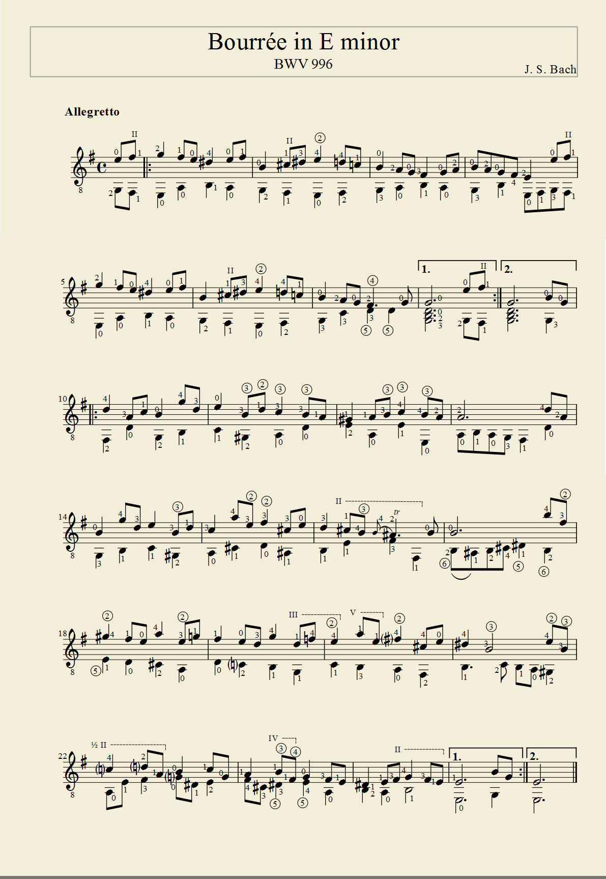
Paul Lutus also used an underlying "canvas" frequency at the verge of human hearing (around 14kHz), and it had a similar effect of being able to put the signal in multiple intermediate states, but in addition to shaping the specific (very characteristic) sound for its Electric Duet, Paul Lutus also employed a mechanism to switch audible frequencies fast enough for the switching itself to escape human attention. The result is a very capable duophonic engine which is small, responsive to computer events without distorting the music, and which can be used in other programs. The notes on the development of Electric Duet provide fascinating insight into the programmer's challenges and writing adventure. And the results are mindblowing; listen to the following piece, Bach's Bourrée in E Minor, played on Electric Duet. It sounds really clean and is such a pleasure to listen to.
When one looks at the musical notation for Bach's Bourrée in E Minor played above, it is immediately obvious that two-voice counterpoints like these, a popular form of baroque music, are perfectly suited for two-voice Electric Duet:
Lastly, here are interesting phantom waves I observed when running my frequency and pulse width modulation program on the Apple IIe hooked up to an oscilloscope. I'm not fully sure what they result from and I definitely need to dig deeper into this; for now let me just put them here for the record. The first gif shows what I observed at approx. 10ms-per-square view when modulating frequency relatively high in the audio spectrum while the second what I observed at a set (again, relatively high in human-hearable spectrum) frequency when modulating the pulse width. My best guess these are standing waves, similar to beat frequency discussed later in ZX Spectrum section, and that they originate in a flaw in my code. I need to dig deeper into this.
ZX Spectrum, for many of us the hated and loved entry point to computing, had a tiny but annoyingly loud speaker built in, and game devs did wonders with it. We won't be discussing basics of square waves, pulse width modulation, etc. again, because these subjects are covered in the Beep and Apple II sections above, and they apply just the same to ZX Spectrum. Also, we will not be discussing the more advanced AY sound chip used in later ZX Spectrum iterations — those will be covered in a separate section. Here, we're focusing on 1-bit output again, but with some attention to the specifics of the ZX Spectrum platform, and on the masterpieces some of the ZX Spectrum developers and demoscene artists have been able to produce using this limited medium. Some the sources of information, and inspiration, for this section were Blake Troise's 1-Bit Instrument article; Kenneth McAlpine's Bits and Pieces: A History of Chiptunes. book; Piotr Marecki, Yerzmyey, Robert Hellboj Straka's ZX Spectrum Demoscene book; and Pavel Lebedev's Мир звуков спектрума (World of Spectrum Sounds).
There is a video accompanying this section, have a look below!
Writing a simple tune made of plain 50-percent duty cycle beeps is easy without machine language skills thanks to the BEEP command available in ZX Spectrum BASIC language interpreter which starts from the computer's ROM. Here is a classic rock melody represented using the BEEP command played in a loop, with pairs of numbers (duration, pitch) fed by READ command from data stored in memory using DATA command:
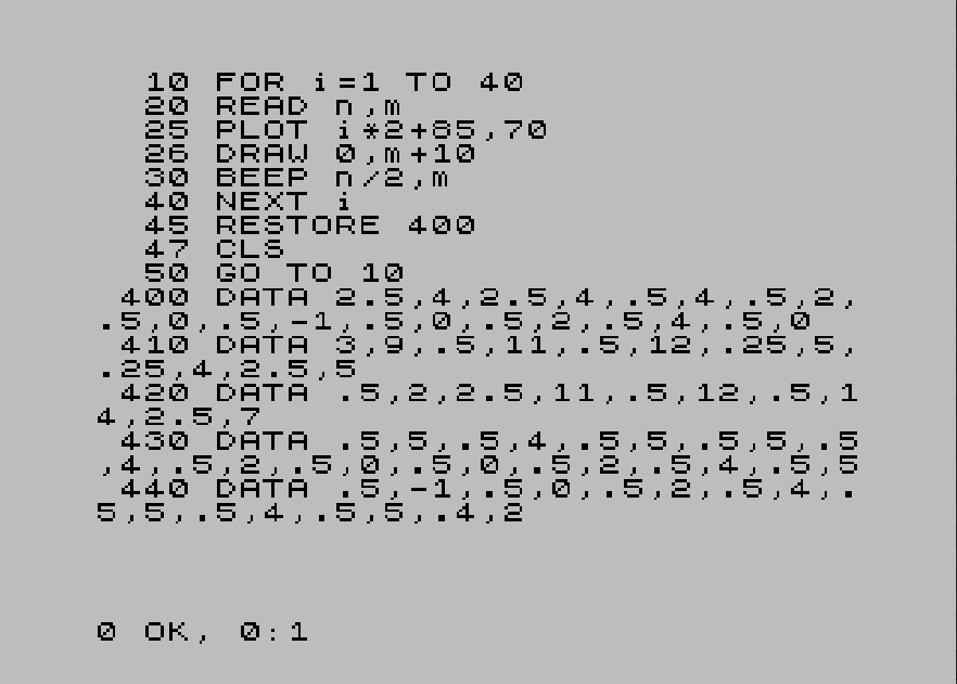
If you ever happen to run that code, you will also see that as well as playing notes, it draws vertical lines corresponding to the pitch of the current note. And the tune sounds like this:
One trait of simple CPU-driven sound generation devices was that frequency and duration — both being dependent on time — were tied to the CPU's precise frequency. We saw that in the Apple II section above where the difference between PAL and NSTC versions of Apple II made a difference in sound frequency. In ZX Spectrum the difference is even more pronounced when we look at how two variants of the computer, ZX Spectrum and ZX Spectrum +2. The former is clocked at 3.5MHz while the latter at 3.5469MHz, plus there are other timing differences, all of which cause the same BASIC code to play at slightly different frequencies and with slightly different timings. Timing peculiarities are the result of ZX Spectrum being a real-time computing device whose software operation is tied to CPU speed. Listen to how these two computers start at the same time, but diverge more and more as the melody progresses:
I had fun trying to find the right factor to multiply the duration by in the faster ZX Spectrum +2 so that the two tunes are timed the same way, and arrived at x1.015 number which seems to be close enough. Even though I did not have to adjust the timing of the slower ZX Spectrum, I still added x1 factor to the code running on that machine, because I wanted to eliminate from the equation the delay caused by the multiplication operation itself:
ZX Spectrum adjustment:
30 BEEP n/2*1,m
ZX Spectrum +2 adjustment:
30 BEEP n/2*1.015,m
Since the timing adjustment only fixed the sound duration, but not the differences in sound frequencies, when the adjusted code is played side by side from both computers, we can hear a very pleasing detune/unison effect:
It is worth noting that the pitch values corresponding to C major scale given in most ZX Spectrum BASIC programming textbooks (C = 0, D = 2, E = 4, F = 5, G = 7, A = 9, H = 11, C = 12) are only approximate, and need to be adjusted to match the specific CPU. In his article Мир звуков спектрума (World of Spectrum Sounds), Pavel Lebedev gives the following values to correspond to C scale notes: C = 0, D = 2.039, E = 3.86, F = 4.98, G = 7.02, A = 8.84, H = 10.88, C = 12. Listen below to what the difference sounds like for the sound E on a ZX Spectrum. It is pretty audible. These values, valid for a ZX Spectrum, will of course not work for ZX Spectrum +2A for the reasons described above.
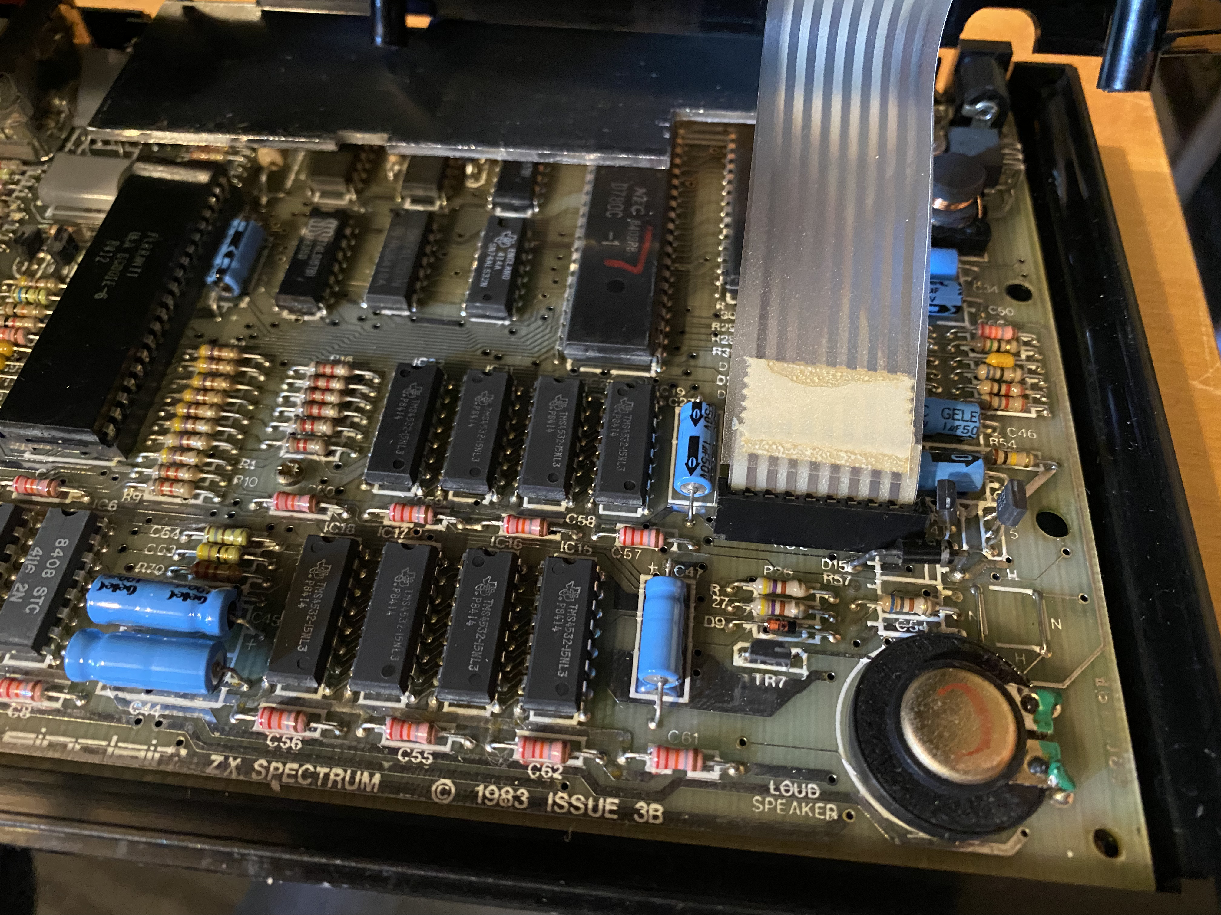
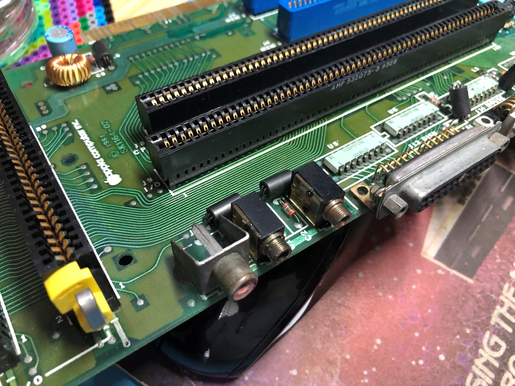
Now, before moving on to more advanced ZX Spectrum sound techniques, let us expand a little on the question we asked when discussing Apple II: why a square wave does not really look square. In ZX Spectrum it is even more clearly demonstrable, and we need to get this subject out of our way before we dive into more detail; otherwise some of the oscilloscope readings may puzzle us. The original ZX Spectrum can output sound either via the built-in speaker, or via a 3.5mm EAR or MIC (ZX Spectrum 16/48K/+) or TAPE/SOUND (ZX Spectrum +2 and higher) socket. If we look at the schematics, it is clear that there are many more capacitors and resistors on the path from the ULA chip (which switches the speaker on and off) to the EAR and MIC sockets than there are on the path to the speaker. In case of the speaker, the signal from ULA goes straight to a transistor which applies (or disconnects) 9V voltage to the speaker. As for whether to choose EAR or MIC, even though there are differences in how EAR and MIC sockets are driven, and the levels of output on each of them, for the purposes of this article we can consider them equivalent; for my experiments the amplifier was connected to the MIC socket. In any case, for either EAR or MIC there are a couple of capacitors and resistors on the way which degrade the rectangular signal; that degradation does not affect audible qualities (actually the amplified signal sounds much better than via the tiny speaker), but it affects the shape of the wave as displayed on the oscilloscope, and skews our experimentation. Here is what it looks like in practice: check out this simple BASIC code which plays a high-pitched 0.1s sound, pauses for 1/50th of a second, plays the sound again, and so on ad infinitum.
10 BEEP .1, 20
20 PAUSE 1
30 GOTO 10
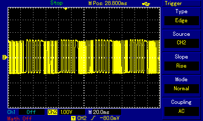
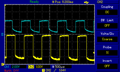
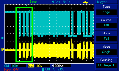
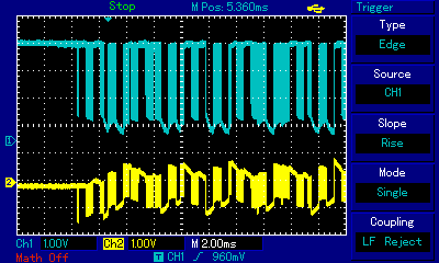
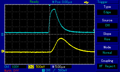
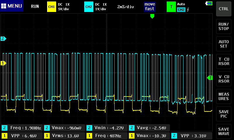
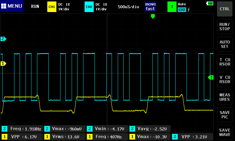
If we look at the oscilloscope representation of the sound produced by this program, we can see the differences between where we actually measure the signal. In the images below, showing a single square pulse and the entire 0.1s pulse train respectively, blue line represents the signal as coming from the ULA chip (probe connected directly to the chip pins) or as measured at the built-in speaker (the singals looked the same), while the yellow line represents the signal in the 3.5mm socket.
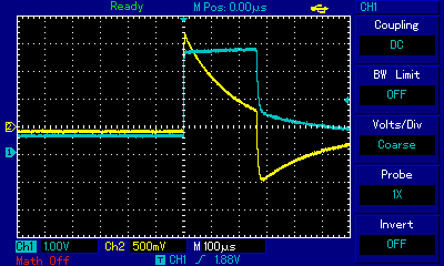
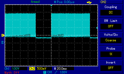
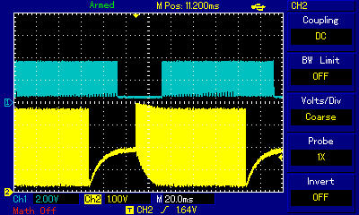
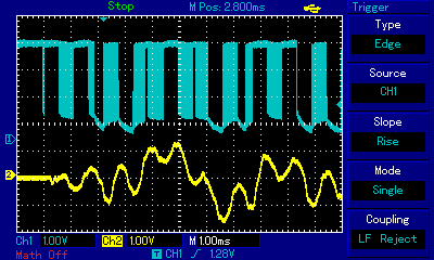
When looking at a single pulse, the signal from ULA is by no means an ideal rectangular wave, but it much closer to ideal square than the one measured at EAR socket. But perhaps even more important difference can be seen at pulse train zoom level where one can observe the buildup and release of signal level over time as pulses are output one after another. That phenomenon, again related to extra capacitance along the signal path, can only be observed at EAR/MIC socket (yellow), and is almost absent at direct ULA measurment (blue). For added perspective, here is signal measured at socket in ZX Spectrum +2 compared to direct ULA measurment in ZX Spectrum 48. Examine how the socket (labelled TAPE/SOUND in ZX Spectrum +2) behaves much "better" regarding rectangular wave representation; at pulse zoom level the signal is almost identical to the one measured at ULA; only at pulse train level zoom do we discover that the signal is pushed to higher overall level first, then gradually resumes a stable level after a couple dozen consecutive pulses.
As discussed in section Apple II earlier, the imperfections of square wave representation, in particular the time delays in reaching the high/low levels of subsequent electronic components, are one of the means to build more advanced polyphony techniques used by 1-bit artists. Let's re-visit the subject now with ZX Spectrum examples where those techniques have been mastered and where they developed into in an entire demoscene which has persisted until this day despite the demise of ZX Spectrum as a viable general-purpose computing platform. Let us revisit the Maple Leaf Rag piece again, this time as interpreted by Richard Swann in his 48 Funk Box demo. Here is the piece, and it sounds amazing:
Let's pay particular attention to the first three chords:
If we look at Scott Joplin's original score, it is clear that the demo's author chose to play only 2 tones of the 5-tone chord.
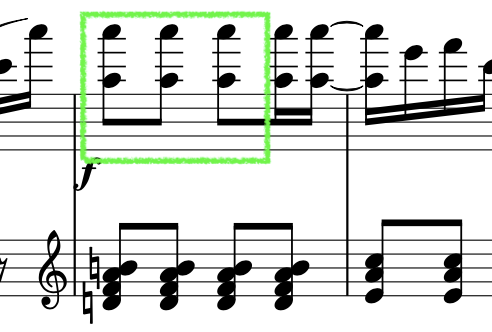
The three 2-tone intervals are represented as the first three blocks of train pulses:
When we zoom in on one of these intervals, we see a pattern of pulses similar to those we studied in the Apple II section:
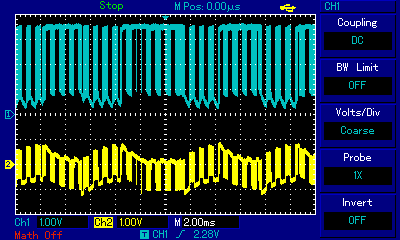
In the earlier Apple II section we explained how pulse width modulation technique is used to overcome the limitation of just two speaker states (in or out) and artificially create intermediate states by carefully modulating very fast rectangular pulses. Let us now observe how (be it with PWM technique or not) the signal conduit all the way to the speaker behaves in our ZX Spectrum-specific setup which we built to mitigate the disfiguration of rectangular waves, with the oscilloscope probe connected directly to the ULA chip. Look at the oscilloscope view below which represents the wave shapes of one of the first three intervals of the above as measured at three points: directly at the Ferranti ULA chip, at the output of the MIC connector, and after amplification at a large speaker (with soundwaves picked up by a microphone):
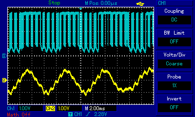
These two images llustrate the gist of 1-bit polyphony techniques: note how the blue graph, representing the signal directly at ULA chip pins, is binary: either high or low state (barring some imperfections of the square wave visible at the bottom as slanted lines). This is what the machine code, and consequently the CPU, generates: carefully timed 1s and 0s. We observe the impulses almost immediately after they have been born, so the entire pulse train has a rectangular shape. The second stage of our observation is different: the yellow graph in the left hand-side image represents the same signal, but much further down the stream: after it left the MIC connector on the back of the computer. It is not rectangular anymore; one can observe undulation! While the detailed shape is still rough, already slopes, peaks and roughs can be discerned. Why is this happening? As explained above, the EAR/MIC socket is not connected directly to the ULA chip: on the way there are resistors, capacitors and a transistor which opens/closes the flow of current to the EAR/MIC connector. All these components, plus the wiring, have their capacitance which translates to signal inertia: it takes time to bring the signal fully up or fully down. By carefully timing signal switching, including modulating the pulse width and/or the number of pulses, 1-bit music developers are able to use that inertia to their benefit and shape the resulting undulation. At this level individual rectangular pulses are still visible, but it is the overall shape of the pulse train that starts dominating in macro scale: a new audible wave is being created. The end effect can be seen in the right hand-side image, where the yellow graph represents what a microphone standing next to a speaker picks up, and which we can use as a proxy for what a human ear receives. There are no individual 1-bit pulses anymore, because the amplifier wiring and the speaker membrane have added even more inertia on top of the components inside the ZX Spectrum. We now see a fully analog audible wave! From function and wave theories, in particular from Fourier transform we know that a polyphony sound wave is a sum of the waves of constituent notes. The two notes of Maple Leaf Rag chords, transposed to A3 and A5, can be seen here as the sum of the lower note (the slower and wider undulation with just 2 peaks visible in the image) and the higher note (the faster and finer undulation with as many as 10 peaks visible in the image), respectively. This is how ZX Spectrum devs and musicians achieve the impossible: represent polyphony using just one channel and 1 bit of resolution.
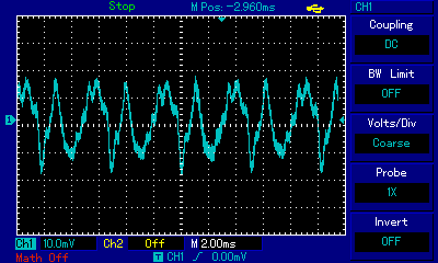
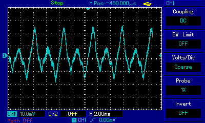
Let's have a look at another example. Here is the intro tune to Sanxion game, 48K version. Let's ignore for a moment the greatness of this piece (originally written by Rob Hubbard for the Commodore 64, transformed to ZX version by Wally Beben), and focus on the very last bars where the melody reaches the highest registers (starting at about 1 minute into the recording):
Here the achieved polyphony is visible even better than in the previous example, with clear separation of the high-pitched final notes (fine wave in yellow in the right hand-side image) from the bass buzzing (larger undulation in yellow the right hand-side image).
ZX Spectrum 48's built-in BEEP command does not provide enough control, or enough speed, to effectively execute polyphony experiments, so let's see how this can be achieved in machine language by looking at the following assembly examples. I used pasmo cross-compiler to build the examples, and then run them on real ZX Spectrums. Let's start by visualizing the very quantum of rectangular wave sound, i.e. the flip between two only possible states, on and off. In ZX Spectrum architecture this is achieved by flipping a bit on the 4th bit of a certain value from 0 to 1 or from 1 to 0 and sending that value to output port 254:
This is what that single flip sounds like:
And let's immediately compare it with two subsequent flips, one right after another:
Listen to what these two flips sound like; they were recorded at exactly the same volume as the single flip above.
The dramatic decrease in volume results from what we discussed before: the inertia of electronic components and the speaker itself which is unable to reach the full "in" or "out" position before the next flip is executed. Compare the oscilloscope view of both pieces of code above:
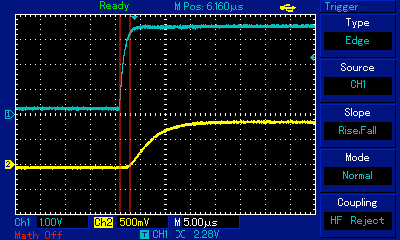
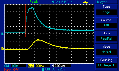
This simple exercise is already allowing us to make a few interesting observations. First, notice how long it takes between ULA sets the signal to high (left hand-side red line in the first image) to when that flip starts occuring at the end of the cable running from the MIC connector (right hand-side red line in the first image). That's already a 2µs (microsecond) delay which will only increase before the signal reaches the amplifier and the speaker, and before the speaker's cone moves. Second, notice how slow the yellow line is to rise to the high level compared to the blue line. This is the result of the capacitance and inertia we talked about earlier. Next, examine the two red lines in the right hand side image which represent the time span between the first flip of the signal (line 3 in the second piece of code above) and the second one (line 5). The ZX Spectrum+ which I used for this experiment has its Zilog Z80 CPU clocked at 3.5MHz, i.e. it performs 3.5 million cycles ("T-states") per second. That's 0.28µs per cycle. The XOR instruction performed after the first flip takes 7 cycles to complete, and the OUT instruction following it takes 11 cycles to complete. The total of 18 cycles equals 18 * 0.28µs = 5.04µs which is the distance we see between the two red lines above! Lastly, compare the yellow lines between left and right images. When we flip once, the yellow line reaches — albeit with a delay — the high signal level, here corresponding to approx. 1V of potential difference. However, when we flip in a quick succession, even though the blue line goes all the way to the high level, the yellow one never reaches the highest state, and starts falling once it has barely touched 0.6V level. The yellow line (MIC line signal) is slower, has lower amplitude, and has smoother shape. Lower amplitude corresponds to lower volume, and the relative slowness and smoother shape allow programmers to cheat the human ear into believing it is hearing analog sound waves.
Also, observe how the selection of machine language instructions can influence the timings, and the resulting sound: if we change the XOR instruction from using a literal (i.e. an absolute value) to a register as an operand...
...then we make the resulting pulse even shorter (total of 15 t-states = 4.2µs):
To build a note out of these ticks, one needs to create series of them long enough to simulate a sound wave. We covered this when experimeting with Arduino earlier in the article. One caveat specific to ZX Spectrum is that to achieve clean-sounding note, one needs to disable interrupts; otherwise the sound is distorted. Listen and compare:
The choppy sound of the first sample above is very characteristic of ZX Spectrum; this "blip-blop" sound is often heard when music is accompanying game/demo execution, or if the program needs to be responsive to interrupts for other reasons. The blip-blop sound is by some considered the trait of ZX Spectrum music, and is often used in creative ways, for example in the following interpretation of Bryan Adams's "Summer of 69" made in 2011 by Gasman/Hooy-Program using Romford engine (we will be covering 1-bit engines shortly). As the authors of the demo track admit themselves, "it sounds crappy because it's entirely using the ROM BEEP routine (...) and leaving 50% of CPU time free for visuals".
Knowing the above, creating a simple one-voice melody is trivial, so instead of describing that let's spend some time on coding for polyphony. In Pavel Lebedev's article which we mentioned before, he shows the following simple polyphony solution which I adapted for this article and programmed to play a simple chord progression of C G A F:
Here is what it sounds like:
The above code is a possible implementation of pulse interleave method (PIM). The premise is simple: there are two counters, one for each frequency we want to play. When either counter reaches 0, it creates a flip and then the counter is reset and starts anew; the method of arriving at a frequency by using counters of loop iterations is akin to dividing one oscillator's frequency to arrive at different notes, and is referred to as divide-down or frequency divide synthesis. Since each counter decrements independently, the speaker flips are also independent and — with some distortion caused by pulse collisions — create two distinguishable voices. Of course the devil is in the detail and as much depends on the values of the counters as it does on all the instructions performed in the two loops: the developers need to be careful about the timing of each instruction counted in T-states, about possible branches taken, location of counters/values in memory, and much more. As an example of real-world implementation of the technique, listen to the intro tune of Manic Miner written by Matthew Smith in 1983:
I used an online tone generator to find the values for d and e above. If you want to experiment with this, you may also try detuning the values by 1 or 2 (either d or e but not both) to create slightly more natural sounding harmonies (perfectly calculated harmonies have an unpleasant ring to them). Or you may want to enjoy the detune effect itself by playing two similar but not identical notes simultaneously, e.g. d = 244, e = 245. What we previously achieved using two ZX Spectrums, can now be reproduced with just one:
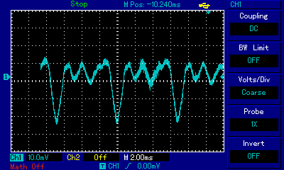
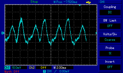
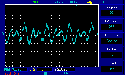
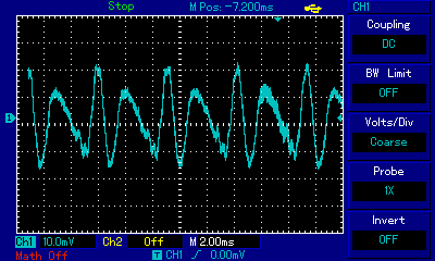
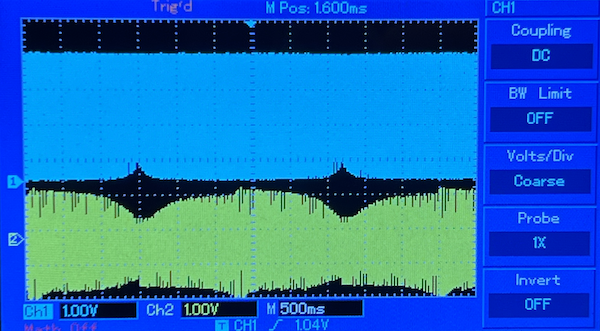
This effect, when plotted on an oscilloscope, is mesmerizing:
The two parallel notes are close to 90Hz, but separated by a fraction of hertz, maybe by 0.5 hertz or so. When they play close to unison, i.e. when the waves are in phase, they look like an almost perfect square wave on the ULA pins (blue line), the amplitude is the highest on the MIC output (yellow line), and the audible underlying "buzzing" is the loudest. On the other hand, the further the waves go out of phase as the time passes, the more "overlapping" of similar-frequency waves we see which in the video above can be observed as "thicker and thicker" switches between high and low; of course they are not thicker, it's just accumulation of densly spaced pulses which result in very fast switching between high and low, and consequently in the lowering of the perceived signal's (yellow line's) amplitude resulting from signal inertia which we described earlier:
If you listen closely to the audio sample above, preferably via an amplifier and big speakers, the deep undulation — a completely new sound wave — resulting from this detune can be heard very clearly. This phenomenon is called beat frequency or beat note, and it is used both when tuning instruments and for artistic expression where it is also referred to as "sweep effect". To calculate the frequency of that new beat note, we need to subtract one of the simultaneous frequencies we used from another: fb = |𝑓2–𝑓1| i.e. in our case say slightly below 90Hz and slightly above 90Hz which gives us, say, slightly less than 0.5Hz of difference. The period of our beat wave should be slightly more than 2 seconds, which is very much what we observe if we zoom out our oscope view!
Returning to the discussion of polyphony, as we mentioned the approach to achieve multi-voice sound illustrated with the assembly code above is called pulse interleaving method (PIM). It is just one of the approaches developers took to overcome the single-voice limitation of ZX Spectrums (and other 1-bit machines). Other methods included PFM (pulse frequency modulation) where momentary frequencies of a pulse train simulate sound frequency changes; PWM discussed at length in the section on Apple II; PPM (pulse pin method) where individual trains of very narrow pulses are used to delineate their respective frequencies without much risk of collisions due to very low duty cycle; and also combinations of these. Initially these methods were hard-coded into individual games, tunes or demos, but it didn't take long for developers to realize that the methods themselves could be codified and made available independently of the artistic content. That is how 1-bit music engines were born.
A music engine is an independent, modular piece of code which takes an array of note/sound parameters stored in memory and executes hardware commands (specifically in ZX Spectrum: initiates speaker ticks) to reproduce these notes or sounds in an engine-specific way using one of the available modulation methods. Music engines were created already during the golden age of ZX Spectrum gaming, with some early examples including Mark Alexander's Music Box engine from 1985, Odin Computer Graphics's Robin engine from 1985 and Tim Follin's famous 3-channel routine from 1987. But it hadn't been until a quarter of a century later, with the revived interest in vintage platforms including ZX Spectrum, that the demoscene saw an explosion of new engines. Dozens of them were created in 2010s, with utz (aka irrlicht project) and Shiru among the most prolific engine coders. Not only have new engines been created, but also classic ones have been rewritten or reverse-engineered. In addition to different modulation techniques used, and consequently the overall feel of the sound, engines differed by the number of channels, presence of the drum channel, and availability of features including timbre and duty cycle control, envelope control, looping, rest notes, speed control per track or per note, decay/LFO effects, and more. With the growing number of such projects, it has become unwieldy to try out individual engines, and to adapt the content to each new one; most of engines required a specific track notation which had to be hand-coded in machine language. To address this, tracker programs ("chiptrackers") have been built which provide a uniform UI for entering notes and effects across mutliple engines, with additional features such as file management, exporting to machine code or TAP format, as sound files, etc. There are both ZX Spectrum-native trackers such as Alone Coder's Beep Tracker and cross-platform ones which enable coding the music on a Windows or Linux machine before transfering it to the ZX Spectrum, such as Shiru's 1tracker or Chris Cowley's Beepola. After the attempts above to write polyphony directly in assembly language, it is refreshing and liberating to be able to use a modular engine plus a convenient UI to compose ZX Spectrum music. Here is a short piece I wrote in less then an hour, with a catchy beguine rhythm, polyphony, arpeggios, duty cycle control and drums. The track was written in Shiru's 1tracker using introspec's tBeepr engine, and then transferred over to my ZX Spectrum+ as a TAP file:
Pieces like the one above are called chiptunes — musical creations, usually accompanying games or demos and usually made on consoles or computers from the 80s and 90s, and characterized by being written for a specific hardware platform. They are most often associated with specific PSGs, as in Commodore 64 or Atari, but the term is equally applicable to Z80 CPU-specific tunes ("beeper" tunes as opposed to AY-chip generated tunes) playable on a ZX Spectrum. Chiptunes are distinguished creative artifacts demoed, exchanged, and ranked during demoscene parties. The shift of focus from demos (encompassing graphics and sound) to strictly musical productions gave birth to the term "chipscene"; there is even a niche but growing interest in entire albums or EPs recorded in chiptune genre, with Yerzmyey's album Death Squad, Shiru's 1-Bit Music Compilations or Tufty's SPECTRONICA album being examples of productions written largely or entirely on a ZX Spectrum.
At first sight Apple Lisa's sound capabilities are no different from other 1-bit sound generating computers discussed here. It has a speaker which only makes beeps. On closer inspection, there are a couple of differences which deserve a separate section. This section has an accompanying video which you can watch here:
In both Apple II and ZX Spectrum, the speaker was activated by on/off signal driven almost directly by the CPU. Every time the signal switched to high or low, i.e. every time the speaker made a single tick, the CPU had to be engaged. In Apple Lisa, even though we're again dealing with just simple ticks (so basically with a 1-bit Digital to Analog converter and a simple square wave), the CPU does not have to be engaged for every tick. It does not have to be engaged 880 times to play a 440Hz A4 note for just one second. Instead, an entire series of bits is pre-programmed once before sending as impulses to the speaker; once sent and the speaker keeps playing, the CPU is free to do something else. In Apple Lisa this has been achieved using a shift register.
Shift register is a generic method for transforming parallel data to serial and vice versa. It can be used for serial communication, to drive LED displays, and for many other things. In old computers it was even used as memory or to drive a display. The shift register which Apple Lisa uses for sound generation is implemented in MOS 6522 VIA (Versatile Interface Adapter) chip. Lisa has two of those chips, one mainly responsible for disk operations, and the other one mainly responsible for keyboard and mouse I/O. A side job of the latter is to support sound. This is done by first pre-programminig the 6522 to enable continuous shift-out operation controlled by one of its built-in timers, timer 2 (T2). Continuous (or "rotate") shift out works by taking bits 0-7 from the parallel data bus and outputting them in a serial manner on one pin (CB2) continuously, i.e. the most recently output bit goes back to the end of the queue. The frequency of output is governed by clock T2. So the programmer has to set the T2 clock (corresponding to note frequency), the number of rotation cycles (corresponding to note duration), and the pattern of 8 bits (corresponding to shape of pulse train). The moment the 8 bits are uploaded to the VIA chip, rotation starts and the CPU is free to do something else.

The method bears some semblance to how sound is generated in PCs, a subject that we will be covering in this article too. Similarly to Apple Lisa, the programmer just sets the frequency of the Programmable Interrupt Timer and is free to engage the CPU in other activities while the PIT chip is driving the speaker. Shift register is different, however, in that it allows (and requires) the programmer to define the pulse train to output. We will see that this gives a little bit of control over the timbre, albeit not much. PC implementation is also different in the fact that a programmer, if they want to circumvent the PIT, has that ability (by directly setting the state of port 0x61). In Apple Lisa there is no port or memory address wired directly to the speaker; however, there are ways of achieving more control over the bits driving the speaker, notably by continuously controlling the parallel-to-serial conversion (rather than letting the shift register rotate).
Interestingly, MOS 6522 designers are listing sound generation for video games as one of the chip's applications, even though the approach employed in Apple Lisa is different from what 6522 manual advised (Lisa uses the 6522's shift register while the manual advised using Timer 1 to generate series of bits). At least one more computer used the shift register to generate sound in a way very similar to Lisa, and that was a Commodore PET (with very simple additional circuitry as documented in Programming The PET/CBM. The original idea came from Hal Chamberlin, author of the monumental book Musical Applications of Microprocessors, and more about the PET implementation can be read in this informative post authored by the prolific demoscene developer and artist Shiru whose some works are presented in the ZX Spectrum section. Shiru took the concept of shift register-generated sound discussed here to the next level and achieved interesting results, albeit not on Apple Lisa. The concept of shift register, not necessarily implemented in 6522 VIA chip, was also used elsewhere in sound delivery, for example in Atari's POKEY chip to generate noise.
I was able to control a real MOS6522 VIA chip with Arduino and demonstrate the concept of "program once for continuous wave generation". Take a look at the setup illustrated below.
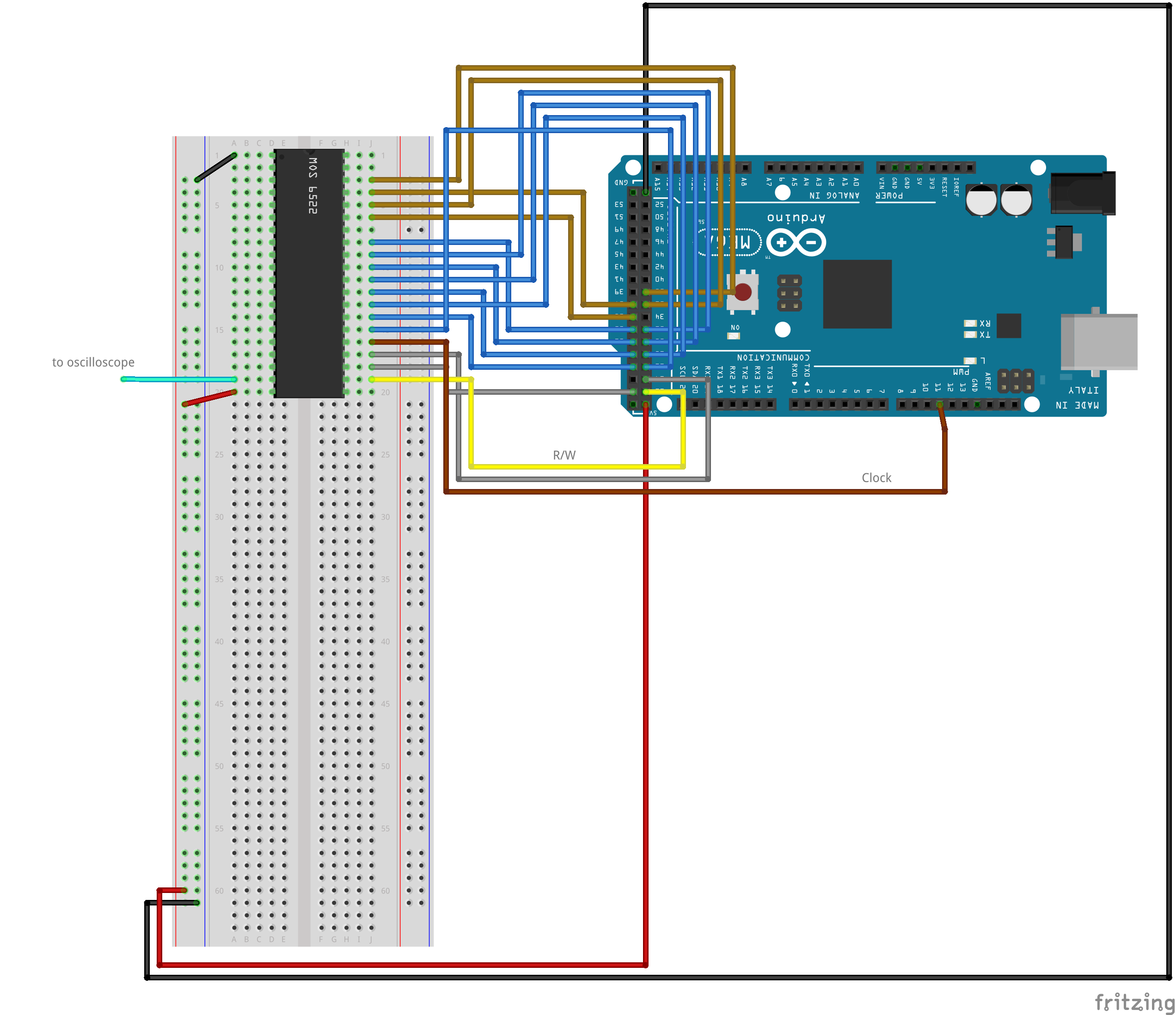
Arduino I/O lines are connected to VIA's data lines and control lines, and a little Arduino program performs the same steps as Apple Lisa to program the chip: 1) Set the Register Select to select ACR. 2) Set the ACR to enable Shift Out free-running mode shift rate controlled by T2. 3) Set Register Select to select T2C-L timer. 4) Set the T2C-L timer to a certain value. 5) Set Register Select to select Shift Register. And 6) Send a wave pattern to the Shift Register (which immediately triggers shifting out). Note that you should not learn from this code: it is primitive and shows my ignorance of the basic microprocessor programming patterns, but all I needed was a proof of concept code to show how 6522, once programmed from Arduino, continues generating the desired waveshape. Full code is under this link, and below only the small fragment which sets the actual pulse train shape.
And after uploading this to Arduino we can observe the following parttern on MOS6522's pin number 19 (CB2 output).
D0-D7 in the Arudino code snippet above.In addition to employing a shift register to generate a pulse train, Apple Lisa has one more interesting solution in its sound subsystem. It allows controlling volume programmatically which differentiates it from the other 1-bit sound capable computers discussed so far (Apple II, ZX Spectrum, PC with a plain speaker). In Apple Lisa, 3 addressable lines designated to control volume via a resistor ladder. Resistor ladder is a circuit in which data lines are connected to resistors arranged in such a way that changing the high/low states of the data lines affects the voltage applied to the circuit. The digital bits, depending on their significance (from the least significant to the most significant) are weighted in their contribution to the output voltage V. In fact, a resistor ladder is a simple digital-to-analog converter (DAC) which, given enough number of bits and precise resistor values, can serve as sound DAC. However, in case of the Lisa, instead of modulating the shape of the sound wave, it modulates it's overall amplitude, i.e. serves as a digital volume controller. The 3-bit resistor ladder used in the Lisa gives a programmer 8 different output voltages to select, i.e. 8 different volume levels.
A very simple circuit shown below, driven by Arduino, illustrates the resistor ladder concept. Arduino's three data lines have been connected to 2 x 220K resistors in series (= 440K) each (these are ladder "rungs") and they in turn are connected on one side (ladder "side rail") with 220K resistors. So for each step the rung resistor value is 2x the side rail resistor value. The reference voltage is here provided by Arduino itself rather than from outside, and an oscilloscope is connected at the most significant bit side of the ladder.
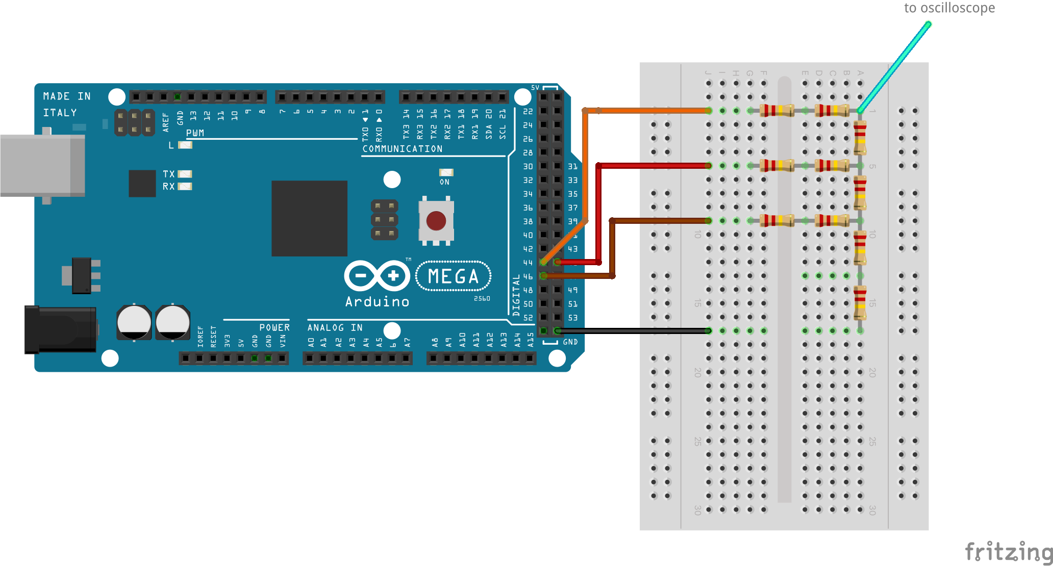
From software side, all we need to do is to set the digital pins in some sequence to test how different digital values get translated into analog voltage levels (below only a fragment exemplifying bit setting, full code here:
The resulting oscilloscope image clearly shows the 8 addressable levels of our makeshift 3-bid DAC.
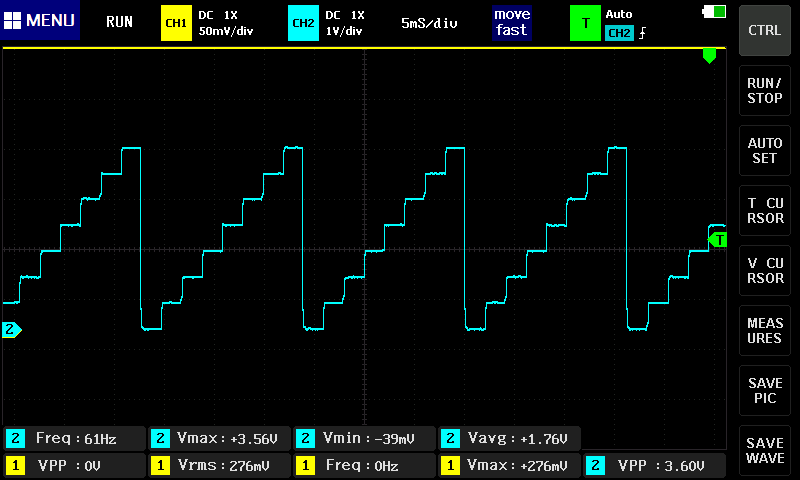
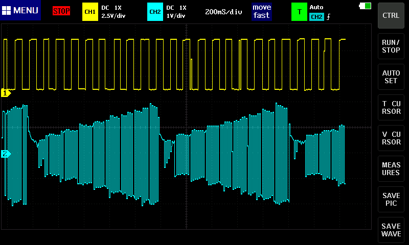
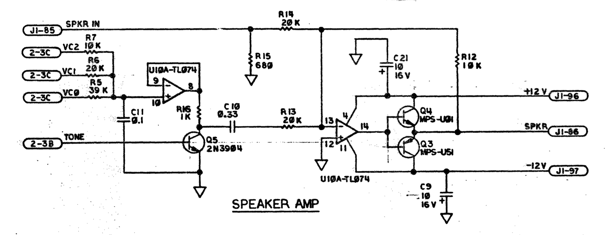
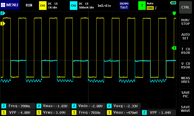
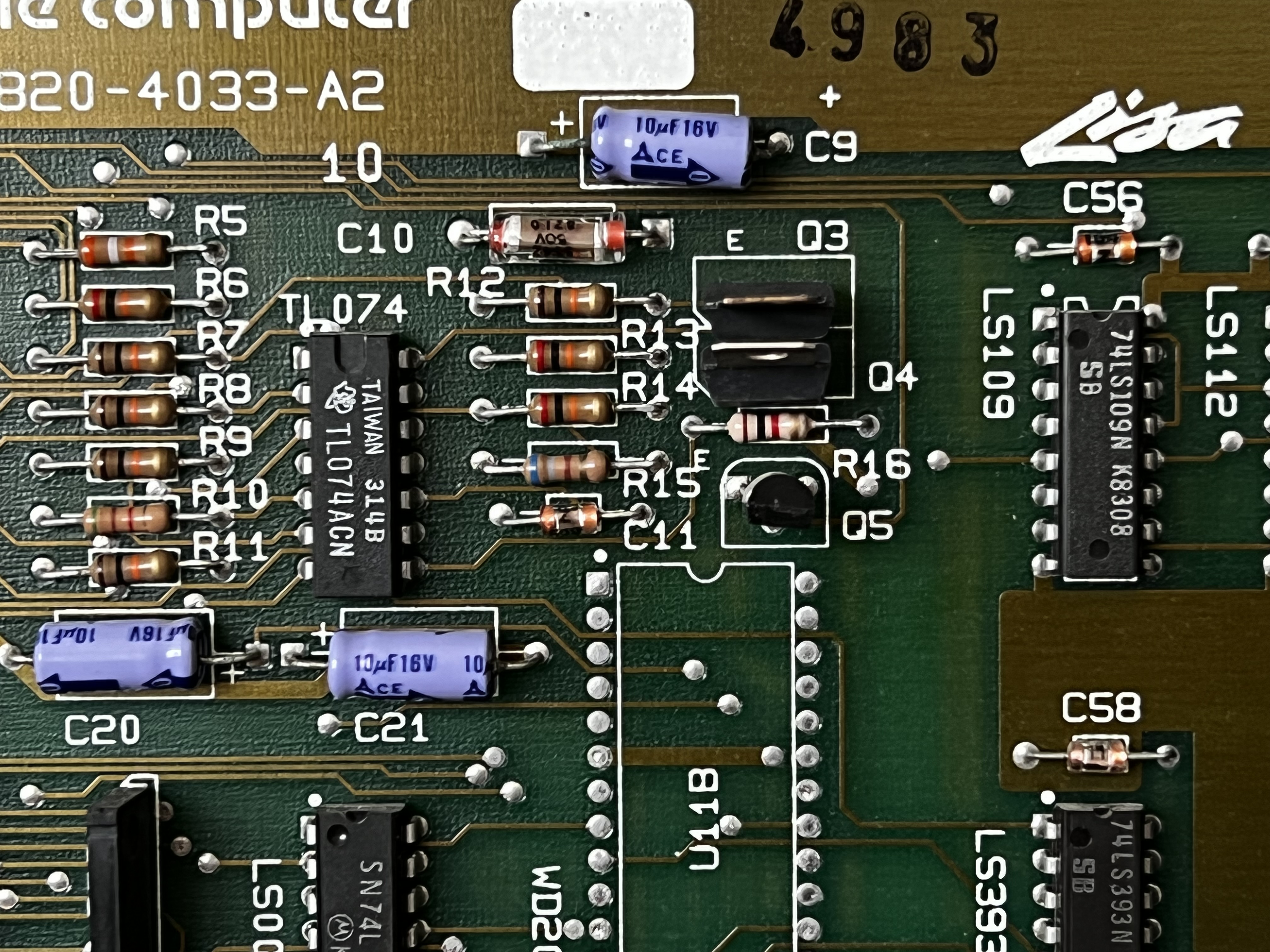
~0V to ~4V), and the delay between changes was 2ms. On the right hand side, signal proped from the Lisa itself: a pattern of 8 notes of the same pitch, 50-percent duty cycle, played in fast succession at 8 different volume levelsAs mentioned, in Apple Lisa this digital-to-audio conversion method is not used to generate the soundwave itself, but to modulate the volume. Voltage modulated by the resistor ladder (left hand side of the schematic below) is enabled/disabled by a transistor controlled directly by the impulses shifted out of the VIA discussed earlier; those impulses control the wave frequency, and the resistor ladder only controls the amplitude. The rest of the circuit is an amplifier based on a TL074 chip which also divides the frequency of the 6522 train by half.
From software perspective, there are several ways to drive the sound hardware described above. One simplest way is to... turn the computer on. Some of the startup test steps are confirmed by short and unpleasant clicks, and then Lisa makes a beep sound if it cannot find a floppy (called minidisk or Twiggy disk in Lisa's parlance) or a hard drive. The clicks and beeps sound like this:
A more controlled way to play sound is to use Lisa's Pascal language interpreter's BEEP command. In Workshop development suite (e.g. Workshop 3.0) one needs to enter Pascal code in the editor, with HWINT library included and with a BEEP command which takes duration and pitch as arguments.
Then compile it with P command to beep.obj, and link it with L command using beep.obj, iospaslib.obj and sys1lib.obj. The object files are linked successfully into an output file, e.g. bp.obj. Then one can run the program with the R command.
The very big change compared to e.g. ZX Spectrum's BASIC implementation of BEEP is the fact that the processor is released to do its next task right after calling BEEP, and as a result in Apple Lisa's Pascal the call to BEEP is not blocking. This means that a call to BEEP right after an earlier one causes overriding the earlier one immediately, regardless of the duration specified in the earlier one. I wanted to code the notes of a Polish nursery tune about a little goat, but to play notes with expected timings I had to introduce additional artificial delays between BEEPs. And because Lisa's Pascal doesn't have a built-in "sleep" or "wait" function, I had to write my own delay procedure which was an educating experience in itself. The whole coding was fun because each time I made a mistake I had to re-compile the code, re-link it, and re-run it which on a 40-year old computer is a lesson in patience and persistence. Check out the finished tune. The code can be found here.
The fact that sound routines in Lisa's Pascal are non-blocking is, of course, a feature not a bug. Note the program below which would be impossible on a ZX Spectrum or Apple II. The program switches the sound on with NOISE instruction which takes only pitch but not duration (and contrary to its name, the function does not generate random noise wave but a regular sound wave), then runs a loop while the sound is playing, and finally switches sound off with the SILENCE instruction.
As for low-level (assembly) coding for Lisa sound, in writing the code samples for this article I received a lot of help on the LisaList2 forum, in particular from Ray Arachelian who authored the Lisa Emulator Project (LisaEm) and from Tom Stepleton, author of many Lisa-related projects, including a beautiful Mandelbrot demo. Without their help I would probably be still stuck in trying to run my first machine code on Lisa — they made the first steps of that journey much easier.
If one wants to go follow the low-level sound coding path, they are responsible for coding the communication with the 6522 VIA chip, that is for setting the correct value to the Auxiliary Control Register in order to enable Shift Out operation, setting the free-running shift out mode controlled by timer 2, setting the actual timer value, and finally sending a pattern to the shift register. The best way to start is to re-use Lisa's built-in ROM implementation of TONE procedures. This helps a lot, because all the constants required for addressing the VIA chip are already set and there is no need to figure them out based on the hardware manual. Similarly this approach allows us to avoid having to define all equates, and re-write shift register access routines in the same way I had to do that for the Artuino project mentioned earlier. The only modification I made was to replace the hard-coded 50-percent duty cycle square wave with a variable which I could set in my score. The rest was fun: I used a frequency tuning app to arrive at pitches for individual notes, and also defined constants for note durations. Below is a working framework in assembly, pre-populated with a few notes, ready to compile and run on the Lisa.
It is now up to the creativity of the programmer to use this framework. Here are a few samples where I experimented with fast arpeggios, pulse train pattern (resulting in timbre changes), and volume (giving an echo effect)
There is a lot more that can be done with the Lisa. The code can be modified to continuously upload new patterns to the shift register (rather than rotating the same pattern over and over again) which would give us access to polyphony and much lower pitches, as well as additional shaping of timbre and volume. In combination with the hardware volume control already available in the Lisa as well as Lisa's much more powerful CPU compared to ZX Spectrum or Apple II, there is a potential here to build a very interesting 1-bit sound platform. Apple Lisa, despite the status of an iconic computer, never built an enthusiast community and demoscene around it because of its very high price and in consequence mostly business, not hobbyist, use. There is only one demo written for Apple Lisa which I'm aware of, Le Requiem de Lisa, but it does not explore the sound aspect beyond simple 50-percent duty cycle square wave melodies. I am hoping that this can be changed in future, especially when the excellent LisaEm emulator is fixed to correctly support sound so that the physical platform is not needed for experimenting.
It is also worth noting here that originally Apple Lisa was meant to have a more advanced sound subsystem. The square wave leaving the shift register via the CB2 pin was not supposed to go directly to the amplifier circuit, but to a CVSD chip which would have then create an analog wave shape based on signals from the VIA. The CVSD chip would have also enabled hardware speech encoding and decoding, and there was even a provision for line in and line out audio jack sockets in the prototype. This has never materialized most likely due to cost constraints (Apple Lisa was very expensive even without that more advanced sound circuit).
| When | What |
|---|---|
| June 1977 | Apple Computer, Inc. releases Apple II with a simple 1-bit speaker |
| November 1979 | Atari, Inc. releases Atari 400/800 with POKEY chip |
| 12 August 1981 | IBM introduces IBM Personal Computer with a simple 1-bit speaker later referred to as "PC Speaker" |
| 23 April 1982 | Sinclair Research releases ZX Spectrum 48K also with a simple 1-bit speaker |
| 1982-1983 | MIDI is becoming de facto standard for exchanging information between instruments and audio devices |
| August 1982 | Commodore Business Machines releases Commodore 64 with SID 6581 |
| 15 September, 1986 | Apple Computer, Inc. releases Apple IIGS which has enhanced sound capabilities thanks to ES5503 chip known from Ensoniq Mirage (itself introduced 1984) |
| 1987 | Roland releases MT-32 Sound Module |
| 1991 | MIDI Manufacturers Association publishes the General MIDI (known as GM or GM 1) standard |
| March 2021 | Adam starts writing this article |